The Impact of Public Transfer Income on Catastrophic Health Expenditures for Households With Disabilities in Korea
Article information

Abstract
Objectives
Previous studies have reported that people with disabilities are more likely to be impoverished and affected by excessive medical costs than people without disabilities. Public transfer income (PTI) reduces financial strain in low-income households. This study examined the impact of PTI on catastrophic health expenditures (CHE), focusing on low-income households and households with Medical Aid beneficiaries that contained people with disabilities.
Methods
We constructed a panel dataset by extracting data on registered households with disabilities from the Korea Welfare Panel Study 2012-2019. We then used a generalized estimating equation model to estimate the impacts of PTI on CHE. A subgroup analysis was carried out to assess the moderating effects of family income levels and health insurance types.
Results
As PTI increased, the odds ratio (OR) of CHE in households that contained people with disabilities decreased significantly (OR, 0.92; 95% confidence interval [CI], 0.89 to 0.94; p<0.001). In particular, PTI effectively reduced the likelihood of CHE for low-income households (OR, 0.85; 95% CI, 0.81 to 0.89; p<0.001) and those who received medical benefits (OR, 0.78; 95% CI, 0.68 to 0.89; p<0.001).
Conclusions
This study highlights the positive effect of PTI on decreasing CHE. Household income and the health insurance type were significant effect modifiers, but economic barriers seemed to persist among low-income households with non-Medical Aid beneficiaries. Federal policies or programs should consider increasing the total amount of PTI targeting low-income households with disabilities that are not covered by the Medical Aid program.
INTRODUCTION
The rapid increase in the aging population without a proper social safety net in Korea has had a significant detrimental impact on the life of people with disabilities and the elderly [1]. The socioeconomic levels of households containing people with disabilities are prominently lower than those of other households. Higher poverty rates are also a widespread problem among households that have members with disabilities since a larger proportion of them have public transfer income (PTI) as a major source of income [2]. Evidence has shown that PTI is effective in reducing income gaps by increasing the disposable income of low-income households containing people with disabilities, regardless of their ability to work. In addition, PTI contributes to eliminating health inequity by lowering the access barriers for those who are unable to visit clinics or hospitals due to financial difficulties [3].
However, while public assistance policies for disabled people have been introduced and gradually improved over the past decades, some argue that these policies have failed to adequately compensate for the medical burden placed on households that have members with disabilities regarding the strict eligibility and low payout rates of the Medical Aid program [4]. Since disabled people are inherently in poor health, they have higher medical burdens than non-disabled people [5]. Understanding the medical burden of households containing people with disabilities to prepare appropriate policies at the national level is critical for achieving health equity across the entire population. Thus, this study aimed to systematically analyze the effect of PTI on the odds ratio (OR) of catastrophic health expenditures (CHE) for households that have members with disabilities.
METHODS
Data
We constructed a panel dataset by extracting data on registered households that had members with disabilities from the Korea Welfare Panel Study 2012-2019 (7th-14th). The selection time for our data was set based on policy changes. The disability pension for severe disabilities and the disability allowance for mild disabilities were revised in July 2010. Hence, data from the 2010-2011 survey were excluded from the analysis, as it was regarded as a wash-out period for policy implementation. Furthermore, the disability grading system was abolished and the severity classification was changed in 2020; therefore, data from the 2020 survey were also not included [6]. Although the current grading system has been simplified, we used the previous grading system for a more granular analysis. Grades 1 and 2 were classified as severe disabilities, grades 3 to 6 were classified as mild disabilities, and unregistered disabled people were excluded from the beginning [7].
The observation period of this study was 8 years from 2012 to 2019, and data were only extracted from households containing at least 1 person with disabilities. In total, 729 households (39.9%) had complete responses to all questions in 8 questionnaires, while 104 households (5.7%) only responded to one questionnaire. The demographic characteristics of the extracted households were represented by the characteristics of each householder. In total, 1050 households were used in the final analysis, and 9706 observations were made, corresponding to 8 years of follow-up of the initial 1369 households.
Independent variables
In this study, PTI was used as an independent variable. PTI was defined as the total personal or household income excluding earned income. We defined it as the sum of annual income from non-contributory public assistance (disability allowance; basic pension; living, housing, or education benefits; childcare allowance; voucher subsidies; etc.) and contributiontype social insurance (public pensions, employment insurance, and industrial accident insurance). To compare households with various numbers of family members, PTI was equalized by dividing it by the square root of the number of household members.
Dependent variables
The dependent variable was the OR of CHE occurrence. We defined CHE based on the method of the World Health Organization (2000; 2005) and Song and Shin [8]. First, we subtracted food expenses (household food, dining out) from disposable income, labeling the resultant outcome as “ability to pay” (y). Disposable income referred to income that can be consumed by consumption and savings among household income, corresponding to the amount that can be used for remaining savings, excluding non-consumption expenditures (such as taxes and medical insurance premiums) from the total income. Next, the proportion of the annual medical burden (T) relative to the ability to pay (y) was calculated (T/y). When T/y exceeded certain thresholds, CHE was regarded to incur [8]. Four thresholds were applied: 40%, 30%, 20%, and 10%. Since various thresholds were used in previous studies, we compared the results of the 4 different thresholds [8]. The annual medical burden included hospitalization fees; outpatient treatment fees; dental treatment fees; payment for operations (including implants, plastic surgery, etc.); and costs for medications, nursing care, postpartum care, checkups, and other health supplements [9,10]. All income and expenses were equalized by dividing them by the square root of the number of household members to facilitate a comparison.
Control variables
The control variables consisted of 3 categories: householder factors, household factors, and year dummy variables. Firstly, the householder factors included gender, age, residential district, marital status, education level, employment status, selfrated health status, underlying chronic diseases, and disability status. Secondly, household factors included the type and grade of disability of the disabled person in the household, family income level, health insurance type, unmet healthcare needs, and the number of disabled and employed people per household. Disabilities were classified into three groups: physical disabilities (encephalopathy, visual, hearing, speech, and facial impairment, etc.), mental disabilities (autism spectrum disorder and other mental disorders), internal organ disabilities (cardiovascular, respiratory, digestive, renal, urinary tract, and epileptic disorders). Disabilities with high medical burdens were ranked, and the highest was selected when people had multiple disabilities. The ranking was set as follows: internal organ disability>physical disability>mental disorder [11]. Grades 1 and 2 were classified as severe disabilities, and grades 3 to 6 were classified as mild disabilities. Unmet medical needs were considered to occur only when economic barriers were involved, as measured with a questionnaire asking whether the respondent or his or her family could not visit a clinic or hospital because of a lack of money. Lastly, 8 dummy variables for the years from 2012 to 2019 were used to reflect annual policy changes.
Statistical Analysis
The research model was expressed as the following logistic regression model.
Yitis the dependent variable that refers to whether or not CHE occurred. xit is the independent variable, referring to the total amount of PTI. α is a constant term, and β is a regression coefficient. ui is an error term indicating unit-specific unobserved heterogeneity for each individual that does not change over time. eit is an error term excluding ui, and it is a value that leaves only the portion of variation according to the individual (i) and the time (t).
Multicollinearity was checked for all explanatory variables before analysis. The average variance inflation factor (VIF) was 1.54, with a maximum value of 2.13 and a minimum value of 1.01, confirming that all variables had VIF values below the reference value of 10.
For the final statistical analysis, a generalized estimating equation (GEE) model was used to reduce the possibility of endogeneity of explanatory variables with a diverse mixture of disability types and grades. This method is also useful for estimating the average effect of the independent variable on the dependent variable as it controls time-varying or non-time-varying variables effectively, thereby reducing systematic modeling errors [12]. The GEE model estimates repeatedly measured parameters by assuming a working correlation matrix that indicates the correlations between the dependent variables [13-15]. An independent correlation structure with the lowest quasi-likelihood information criterion value was selected as the most suitable model for our study [13]. Every analysis used a robust standard error. All statistical analyses were performed using Stata/SE 17.0 (StataCorp., College Station, TX, USA).
Ethics Statement
The authors of this study submitted a research proposal to the Seoul National University Institutional Review Board, and an exemption was approved in October 2021 (IRB No. E2110/004-005). Since we used an open-access source of secondary data, the anonymity of which is guaranteed by using unique personal numbers, the risk of personal information leakage was very low.
RESULTS
Demographic and Socioeconomic Characteristics of Households According to the Presence of People With Disabilities
Table 1 shows the demographic characteristics of the target population and the control group: households with and without disabilities based on the data from the 14th wave (2019). Compared to householders of non-disabled families, householders of disabled families tended to be older, less educated, and unhealthier. Despite their low health status due to overlapping disabilities and chronic diseases, the ratio of employed people per household was higher. They also had lower household income and received Medical Aid benefits more often. The proportion of PTI to household income was higher among families with disabilities (48.3%) than among families without disabilities (26.6%), implying a higher dependency on public assistance among low-income disabled families. Moreover, the proportion of medical burden to the ability to pay was higher among households with disabilities (24.4%) than among households without disabilities (12.1%).
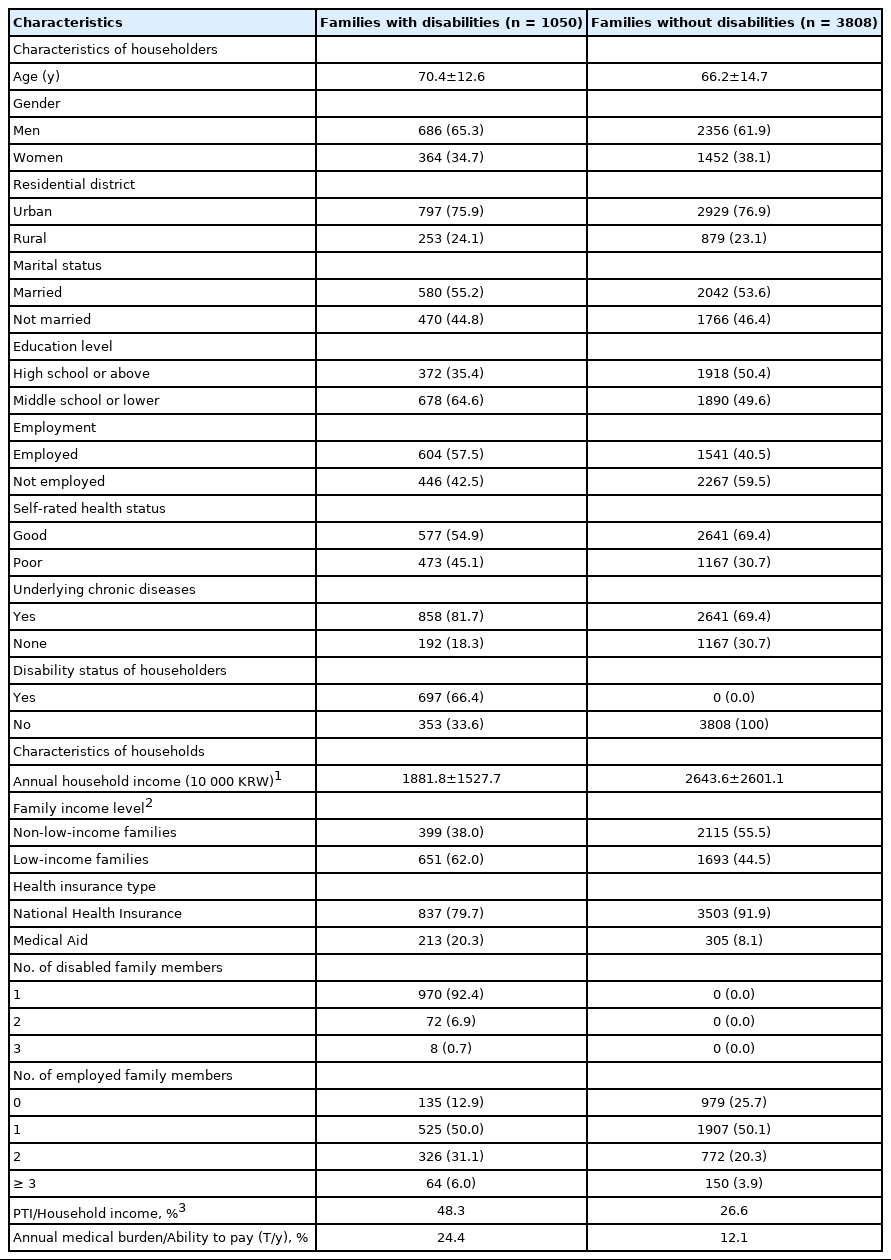
Demographic and socioeconomic characteristics between households with and without disabled members, 2019
Figure 1A describes annual trends in PTI and its beneficiaries among households with disabilities. The amount of PTI gradually increased each year, and the increase was the largest in 2015 when the National Basic Living Benefit system was expanded and reorganized into a customized livelihood, housing, education, and medical benefits system. In contrast, the percentage of beneficiaries remained relatively constant. Figure 1B presents trends in average PTI and medical burden according to the household income quintile among households with disabilities based on the data from the 14th wave (2019). The bar graphs indicate the mean value of total PTI divided by the household income quintile. The line graph illustrates the mean percentage of medical burden relative to disposable income. Higher-income quintiles received more PTI because wealthier families can afford to contribute to social insurance systems, which leads to receiving more income from social insurance pensions. It was also found that receiving a greater amount of PTI reduced the household medical burden. A high medical burden was a key predictor of the occurrence of CHE.
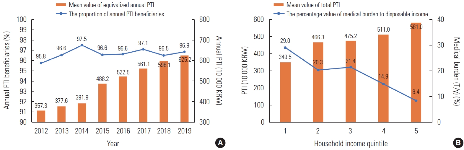
(A) Annual trends of PTI and its beneficiaries among households with disabilities. (B) Average PTI and medical burden according to the household income quintile among households with disabilities (2019). PTI, public transfer income; KRW, Korean won.
Impact of Public Transfer Income on Catastrophic Health Expenditures Using a Generalized Estimating Equation Model
Table 2 demonstrates the GEE results, and a sensitivity analysis was performed with 4 thresholds (40, 30, 20, and 10%). These thresholds were defined by the percentage of the annual medical burden relative to the ability to pay (T/y). When annual PTI increased by 1 million Korean won (KRW), the OR of CHE occurrence decreased significantly at all thresholds: At the threshold of 40%, the OR was 0.92 (95% confidence interval [CI], 0.89 to 0.94; p<0.001), the OR at 30% was 0.94 (95% CI, 0.92 to 0.96; p<0.001), the OR at 20% was 0.95 (95% CI, 0.94 to 0.97; p<0.001), and the OR at 10% was 0.97 (95% CI, 0.96 to 0.99; p<0.001). Our findings proved that PTI had a greater effect on reducing CHE among households who suffer from higher medical burdens.
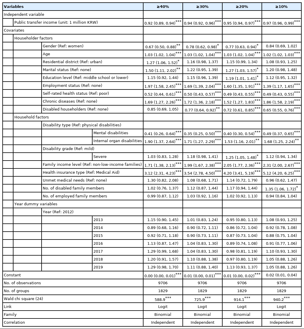
At the threshold of 40%, which indicates the highest proportion of the medical burden, the OR of CHE occurrence decreased among householders who are men (OR, 0.67; 95% CI, 0.50 to 0.88; p<0.01), and householders with a higher selfrated health status (OR, 0.52; 95% CI, 0.44 to 0.61; p<0.001). However, the odds of CHE occurrence significantly increased among older householders (OR, 1.03; 95% CI, 1.02 to 1.04; p<0.001), householders who lived in rural areas (OR, 1.27; 95% CI, 1.06 to 1.52; p<0.05), married householders (OR, 1.50; 95% CI, 1.11 to 2.02; p<0.01), employed householders (OR, 1.97; 95% CI, 1.58 to 2.45; p<0.001), and householders with underlying chronic diseases (OR, 1.69; 95% CI, 1.27 to 2.26; p<0.001). Using households with people who had physical disabilities as a reference group, households with people who had mental disabilities had a lower OR of CHE occurrence (OR, 0.41; 95% CI, 0.26 to 0.64; p<0.001), while households with people who had internal organ disabilities had a higher OR of CHE occurrence (OR, 1.90; 95% CI, 1.37 to 2.64; p<0.001). No statistically significant difference was found between mild and severe disability grades. The most important finding was that the OR of CHE occurrence was about 2 times higher in low-income families than in non-low-income families at all thresholds. Furthermore, compared to Medical Aid beneficiaries, households with health insurance coverage were 3-5 times more likely to experience CHE.
Subgroup Analysis of Catastrophic Health Expenditures Occurrence by Family Income Level
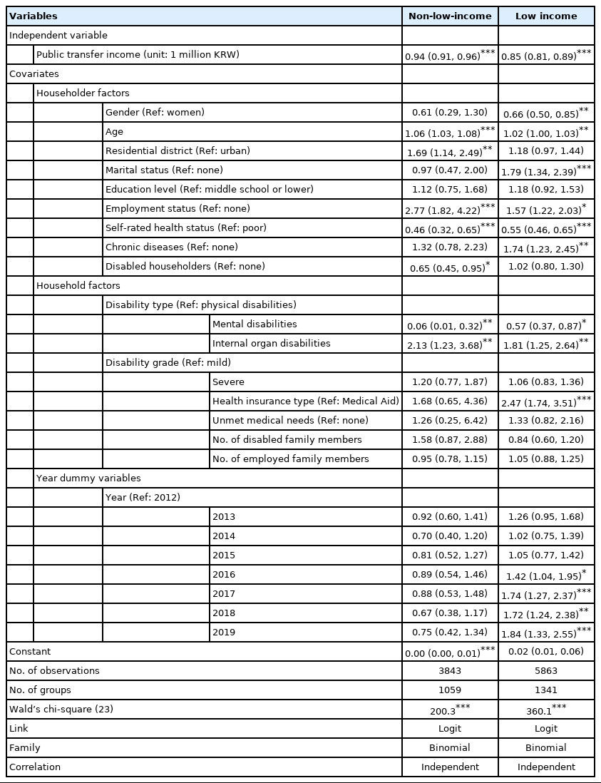
Table 3 presents our findings regarding the effect of PTI on the occurrence of CHE according to family income level, with a cut-off value of 40%. When annual PTI increased by 1 million KRW, the OR of CHE occurrence was 0.94 (95% CI, 0.91 to 0.96; p<0.001) among non-low-income families with disabilities, while the OR of CHE occurrence was 0.85 (95% CI, 0.81 to 0.89; p<0.001) among low-income families. This implies that the effect of reducing the occurrence of CHE due to PTI was greater in low-income households with disabilities. In particular, the OR of CHE occurrence was drastically higher among low-income households with health insurance coverage who could not receive Medical Aid benefits.
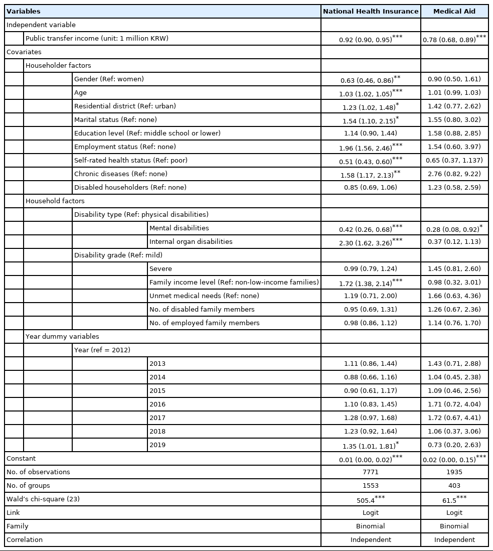
Subgroup Analysis of Catastrophic Health Expenditures Occurrence by Health Insurance Type
Table 4 shows the effect of PTI on the occurrence of CHE according to health insurance type, with a cut-off value of 40%. When annual PTI increased by 1 million KRW, the OR of CHE occurrence was 0.92 (95% CI, 0.90 to 0.95; p<0.001) among households with health insurance coverage, while the OR of CHE occurrence was 0.78 (95% CI, 0.68 to 0.89; p<0.001) among households receiving Medical Aid benefits. The type of health insurance had a moderating effect on the relationship between PTI and CHE occurrence, especially among low-income families. Moreover, households with health insurance coverage experienced CHE occurrence differently among disability types: using households with people who had physical disabilities as a reference, households with people who had mental disabilities showed a lower likelihood of CHE occurrence, while households with people who had internal organ disabilities showed a higher likelihood. However, this result was not replicated among households receiving Medical Aid benefits.
DISCUSSION
In this study, we examined the impact of PTI on CHE, focusing on low-income households and households with Medical Aid beneficiaries that contained people with disabilities. Our findings revealed that PTI had a positive effect on reducing the medical expenses of households with disabilities, particularly low-income families and households with Medical Aid beneficiaries. These results correspond to previous studies finding that low-income households containing people with disabilities heavily rely on PTI [16-19]. PTI promotes the economic independence and stability of households by compensating for the loss of income caused by loss of working ability and other costs incurred by the disability itself.
Most importantly, the family income levels and the type of health insurance appeared to be major moderating factors for CHE. Similar results have also been reported in previous studies [20-23]. Since health insurance coverage covers a relatively low proportion of expenses in Korea, out-of-pocket payments for medical services can be a critical factor causing excessive financial strain on households that are non-Medical Aid beneficiaries. While households with health insurance tended to be wealthier than Medical Aid beneficiary households, economic barriers seemed to persist due to substantial out-of-pocket payments. Furthermore, consistent with previous findings, households with people who had internal organ disabilities had the highest medical expenses, but the severity of the disability was not associated with any significant differences [11].
Based on the study findings, we first suggest that when designing or evaluating policies aimed to alleviate financial distress for households containing people with disabilities, various social determinants of health should be considered. Determinants include household income, the type of health insurance, types of disabilities, and regional disparities [24]. Next, tailored services and support programs must be developed for households with low-income that are not eligible for Medical Aid, which had a substantial proportion of unmet medical needs [25]. Lastly, to fully compensate for essential living expenses and reduce financial distress for households with disabilities, the PTI system must be expanded and the benefit level should be increased [26-28].
There are several limitations to this study. First, the income of households with disabilities may have been underestimated, as the Korean Welfare Panel oversampled low-income households. Second, heterogeneity in disability type and grade may have caused representation issues of the disabled population, which was not sufficiently controlled. Third, the direct effect of PTI on CHE could have been affected by annual policy changes. By utilizing a GEE model, this study attempted to solve the endogeneity problem of explanatory variables and to understand the average effect on each outcome variable. We also conducted an analysis using cluster-robust standard error for household panel ID units to prevent the overestimation issue found in unbalanced panel data. In this regard, future studies should establish a large-scale prospective cohort for each type of disability to conduct a subgroup analysis, and should apply statistical methodologies that better illustrate causal inference.
Despite these limitations, this is the first study to investigate the effect of PTI on the occurrence of CHE by utilizing longitudinal data from about 1050 households with disabilities. The findings of this study contribute to evidence-based decision-making to create a safety net through a plan to expand the PTI system to prevent individuals with disabilities and households with disabled members from falling into the poverty trap.
Notes
CONFLICT OF INTEREST
The authors have no conflicts of interest associated with the material presented in this paper.
FUNDING
None.
AUTHOR CONTRIBUTIONS
Conceptualization: Chang EJ. Data curation: Chang EJ, Kang SC. Formal analysis: Chang EJ. Funding acquisition: None. Methodology: Chang EJ. Project administration: Chang EJ, Jeong Y. Visualization: Chang EJ, Kang SG. Writing – original draft: Chang EJ. Writing – review & editing: Chang EJ, Kang SG, Jeong Y, Kang SC, Kang SJ.
ACKNOWLEDGEMENTS
This paper is based on “The impact of public transfer income on catastrophic health expenditure for households with disabilities”, the lead author’s master’s thesis at the Graduate School of Public Health, Seoul National University.