
Articles
- Page Path
- HOME > J Prev Med Public Health > Volume 55(2); 2022 > Article
-
Special Article
Application of Standardization for Causal Inference in Observational Studies: A Step-by-step Tutorial for Analysis Using R Software -
Sangwon Lee
 , Woojoo Lee
 -
Journal of Preventive Medicine and Public Health 2022;55(2):116-124.
DOI: https://doi.org/10.3961/jpmph.21.569
Published online: February 11, 2022
Department of Public Health Science, Graduate School of Public Health, Seoul National University, Seoul, Korea
- Corresponding author: Woojoo Lee, Department of Public Health Science, Graduate School of Public Health, Seoul National University, 1 Gwanak-ro, Gwanak-gu, Seoul 08826, Korea, E-mail: lwj221@snu.ac.kr
Copyright © 2022 The Korean Society for Preventive Medicine
This is an Open Access article distributed under the terms of the Creative Commons Attribution Non-Commercial License (https://creativecommons.org/licenses/by-nc/4.0/) which permits unrestricted non-commercial use, distribution, and reproduction in any medium, provided the original work is properly cited.
ABSTRACT
- Epidemiological studies typically examine the causal effect of exposure on a health outcome. Standardization is one of the most straightforward methods for estimating causal estimands. However, compared to inverse probability weighting, there is a lack of user-centric explanations for implementing standardization to estimate causal estimands. This paper explains the standardization method using basic R functions only and how it is linked to the R package stdReg, which can be used to implement the same procedure. We provide a step-by-step tutorial for estimating causal risk differences, causal risk ratios, and causal odds ratios based on standardization. We also discuss how to carry out subgroup analysis in detail.
- Epidemiological studies often examine the causal relationship between exposures and outcomes. Randomized controlled trials (RCTs) are a key method for investigating whether a treatment causes an outcome of interest [1]. In an RCT, researchers recruit participants and randomly assign them to either a treatment group or a control group. The results of an RCT are believed to show the causal effect of the treatment for individuals on the outcome. In other words, the estimated treatment effect from an RCT is considered to be unbiased since the random assignment of individuals to treatment and control groups is not affected by confounders.
- Researchers often have difficulty conducting RCTs despite their well-known advantages, since they are generally costly, time-consuming, and prone to ethical issues. For example, physicians would not randomly assign some liver cancer patients to undergo liver transplantation and other liver cancer patients not to receive transplantation. Instead, physicians provide patients with the best treatment option that is most likely to extend their lifetime or cure their condition based on scientific evidence. In addition, if researchers want to conduct an experimental study to determine the effect of a treatment on a disease, financial support and agreements with funders must be secured.
- An observational study is an alternative option for investigating the effects of a treatment on an outcome. However, in observational studies, patients may be influenced by various confounders related to their treatment choices, which results in an estimate of the association rather than causation [2,3]. For example, a study on the simple correlation between coffee drinking and the risk of thyroid cancer would not be able to examine the true effect of coffee drinking on thyroid cancer since the results would be potentially confounded by variables such as age, gender, and socioeconomic status. A high incidence of thyroid cancer among coffee drinkers may be due to an imbalance in variables such as age and gender between the subjects. Even so, the causal effect of coffee drinking on the risk of thyroid cancer can still be inferred through an observational study if certain conditions are met. An advanced methodology known as “causal inference” can be used to estimate causal effects in observational studies. Unlike conventional analysis, causal inference defines the target parameter (i.e., the causal estimand) using counterfactual logic and identifies when the causal estimand can be estimated based on observational data [4].
- Causal estimands may take various forms, including the risk difference, relative risk, or odds ratio. Standardization is a straightforward method for estimating those estimands, in addition to inverse probability weighting [4]. However, compared to inverse probability weighting, there is a lack of user-centric explanations on how standardization can be implemented for estimating causal estimands. Recently, the R package stdReg was developed for implementing standardization, which allows general classes of models, including generalized linear models and Cox proportional hazards models as special cases [5]. This package substantially improves the process of conducting epidemiological studies, and it should be more actively promoted among epidemiologists and public health scientists interested in causal inference. In addition, researchers need to understand how the R package works in order to write an implementation code themselves when the R package is not directly applicable to their models of interest. Therefore, this paper will explain the standardization method using basic R functions only and how it is linked to the R package stdReg. We provide a step-by-step tutorial for estimating causal risk differences, causal risk ratios, and causal odds ratios using standardization. We also discuss how to carry out a subgroup analysis in detail.
INTRODUCTION
- Potential Outcome and Causal Estimand
- Consider 2 random variables. One is the dichotomously measured treatment variable T (1: treatment, 0: no treatment), and the other is the dichotomously measured outcome variable Y (1: event, 0: no event). YT=1 and YT=0 are defined as the outcome variables that would be observed under treatments T=1 and T=0, respectively, and they are referred to as the potential outcomes [4]. For simplicity, we will use YT=1=Y 1 and YT=0=Y 0.
- The population causal effect of treatment exists if Pr[Y 1=1]≠ Pr[Y 0=1], with Pr representing the probability [4]. A measurement of a causal effect answers the question, “What is the outcome if everyone is treated or untreated?” Meanwhile, a measurement of an association answers the question, “What is the difference between the treated group and the untreated group?” The causal effect is determined by measuring the effect of treatment on the same population, whereas the associational effect is determined by measuring the effect of the treatment on 2 different subpopulations.
- The causal effect can be represented by several measures such as the causal risk difference, causal risk ratio, or causal odds ratio (Table 1). The causal risk difference is often referred to as the average treatment effect (ATE). The causal treatment effect is usually identified from RCTs rather than observational studies since the participants in observational studies are not randomly assigned to treatment groups. In order to confirm this, the reasons why measures of association from RCTs indicate causation must be understood.
- Randomized Experiments and Causal Effects
- If researchers randomly assign individuals to receive treatment T, then the potential outcome should be independent of the treatment T, which is expressed as Y 1┴ T and Y 0┴ T. This means that the potential outcome Yt would be equally distributed in both treatment and non-treatment groups. Thus, the subjects in both the treatment and non-treatment groups are considered exchangeable.
- In many cases, the potential outcome is naturally linked to the observed outcome Y as Y=Y 1 for the treatment group and Y=Y 0 for the control group. This condition is known as consistency in the literature on causal inference [4]. In our binary case, the consistency suggests Y=Y 1×1(T=1)+Y 0×1(T=0), with 1( ) representing the indicator function that results in 1 when the event in the parentheses is true. Note that, although Y 1┴ T and Y 0┴ T, Y is not independent of T in general. Under randomized assignment and the consistency condition, the probability that Y t=1 is equal to the probability of an observed outcome for individuals who receive treatment T=t, since Pr[Y=1|T=t]= Pr[Y t=1|T=t]=Pr[Y t=1]. Therefore, the measure of association from an RCT becomes the corresponding causal measure.
- Randomization can be undertaken according to the specific characteristics of individuals, and this approach is referred to as a conditional randomized experiment. For example, doctors may want to measure the causal effect of regular vitamin C supplement consumption (vitamin C=1, placebo pill=0) on the probability of developing of lung cancer (lung cancer =1, no event=0). They can choose to recruit random participants depending on their smoking status (smoker =1, ex-smoker =2, non-smoker =3). In this case, the potential outcome would be equally distributed between a group of smokers who take vitamin C supplements and a group of smokers who take a placebo pill. The vitamin C and placebo pill groups are no longer exchangeable, but they are exchangeable within each stratum for smoking status. This result from the conditional randomized experiment implies that Pr[Y=1|T=t, C=c]=Pr[Y t=1|T=t, C=c]=Pr[Y t=1|C=c], with C representing smoking status. In the above equation, the key condition maintained from the conditional randomized experiment is Y t┴ T |C, which is referred to as “conditional exchangeability” in the causal inference literature [4]. The conditional probability Pr[Y t=1|C=c] provides all of the necessary quantities for evaluating the causal measures described in Table 1 since Pr[Y t=1]=∑c Pr[Y t=1|C=c] Pr[C=c]. This connection is called standardization, which is explained below in more detail.
- Identification
- Valid causal inferences from observational studies can be made if the study mimics a conditional randomized experiment. In other words, within subpopulations with the same set of confounders C, if an observational study is similar to an RCT, the causal effect from observational data can be inferred. In this case, the primary condition needed for making a valid causal estimate based on an observational study is the conditional exchangeability Y t┴ T |C. If the conditional exchangeability from an observational study is maintained, the causal effect of the treatment can be identified from observed data using Pr[Y=1|T=t, C=c]=Pr[Y t=1|T=t, C=c]=Pr[Y t=1|C=c] in the same manner as in a conditional RCT. However, since the potential outcome is not fully observed in an observational study, the conditional exchangeability for each researcher’s application cannot be confirmed. Therefore, expert knowledge is needed to confirm whether the conditional exchangeability is plausible.
- Expert knowledge is commonly believed to be most easily communicated using simple visual representations. A direct acyclic graph (DAG) is one of the most intuitive methods for graphically depicting the causal relationship between treatments, potential outcomes, and covariates. A DAG depicts the direction of the effect of each variable on target variables and helps to determine if covariates C need to be adjusted as well as identifies potential biases such as selection bias, collider bias, and confounding bias [4,6–8]. Shrier and Platt [8] elaborated on the specific steps for building a DAG. Fortunately, there is software for selecting the confounder set C based on causal DAGs. For practical information, researchers can visit http://www.dagitty.net/.
- In addition to the conditional exchangeability and the consistency conditions, the probability of being assigned to either treatment group according to the values for covariate C must be greater than 0. In other words, Pr[T=t|C=c]>0 for all values in c with Pr[C=c]>0. Positivity guarantees that the causal effect can be assessed within the subpopulation if C=c. If the positivity condition is violated in some cases in which C=c, the subpopulation with C=c can be removed from the target population for evaluating the causal estimand of interest. Positivity can be violated in 2 ways: structural violations and random violations [4,9]. Structural violations can occur if the treatment cannot be assigned to individuals under certain conditions. For example, when doctors assign treatment Y to individuals with C=1, the positivity has been structurally violated. Random violation can occur if the 0 event of treatment randomly occurs within the strata of treatment and covariates when the probability within the population is not actually 0.
- Standardization
- An epidemiological study usually aims to establish evidence for implementing public health interventions. For example, if the ATE of vitamin C on lung cancer incidence suggests a preventive effect, campaigns to promote vitamin C intake should be recommended. Standardization is a method for estimating the causal estimand of treatment T on outcome Y in a conditional RCT. The probability of the potential outcome is the weighted average of the probability of the potential outcome according to the values for covariate C weighted by the proportion of the population in C=c for all subjects in c (Pr[Y t=1]=∑c Pr[Y t= 1|C=c] Pr[C=c]). The probability of the potential outcome can be replaced with the observed outcome according to the conditional exchangeability and consistency: Pr[Y t=1]=∑c Pr[Y=1| T=t, C=c] Pr[C=c]. Table 2 shows the method of estimating causal estimands based on standardization.
- Using the standardization method, once Pr[Y=1|T=t, C=c] is evaluated, the causal estimand can be straightforwardly computed since Pr[C=c] can simply be replaced with 1/n, with n representing the sample size. Pr[Y=1|T=t, C=c] can be obtained using logistic regression analysis with Y as a response variable and T and C as the covariates. For different types of Y, other generalized linear models or machine learning techniques may be used.
- The causal effect of treatment in specific subgroups offers important evidence for determining the target populations of public health interventions. In these cases, standardization can be applied to each level of the variable S which classifies the subgroup of interest, in which S contains s groups. For example, if the conditional exchangeability of the subgroup remains S=1, the ATE of treatment T on Y for the subgroup S=1 can be estimated using ∑c Pr [Y=1|T=1, C=c, S=1] Pr[C=c|S=1]– ∑c Pr[Y=1|T=0, C=c, S=1] Pr[C=c|S=1] (Table 3).
- There are 2 methods for estimating the causal effects on subgroups using standardization. The first method is to fit a regression model and evaluate the estimand of the dataset separated by variable S in each subset. Therefore, variable S would be excluded from the regression model. The second method is to fit a regression model including interaction terms with the variable S using the whole dataset and compute the estimand for each subgroup. The choice of the estimation method depends on the sample size of each subgroup. If the sample size of each subgroup is small, then the second method would be preferable since the regression model may not guarantee stability of the fitted model for a small sample size. However, if the sample size is large enough in each subgroup, the first method would be preferred since it would provide a more flexible method for estimating the causal effect of a subgroup since different models can be fitted for each subgroup. Therefore, the bias-variance tradeoff must be considered when selecting the method for estimating the causal estimands of individual subgroups. The estimate using the second method usually results in a more biased but less fluctuating treatment effect estimate than the first method, whereas the first method usually results in a less biased but more volatile treatment effect estimate.
REVISITING THEORY
- This section provides a step-by-step tutorial on how to perform the analysis using the standardization method. The goal in the example is to estimate the average causal effect of initial liver cancer treatment modality on 3-year survival. We used synthetic data that was generated based on Liver Stage Data (LSD) from Korea. The LSD is a sample cohort composed of randomly selected liver cancer patients registered in the Korean Central Cancer Registry between 2008 and 2016 [10]. The LSD includes 10% of newly registered liver cancer patients in Korea, and synthetic data (liver_syn_data1) were generated in this study using the synthpop package in R 4.0.5. The syn function enabled the generation of synthetic data that mimicked the LSD [11], allowing it to be made available to the public without confidentiality concerns.
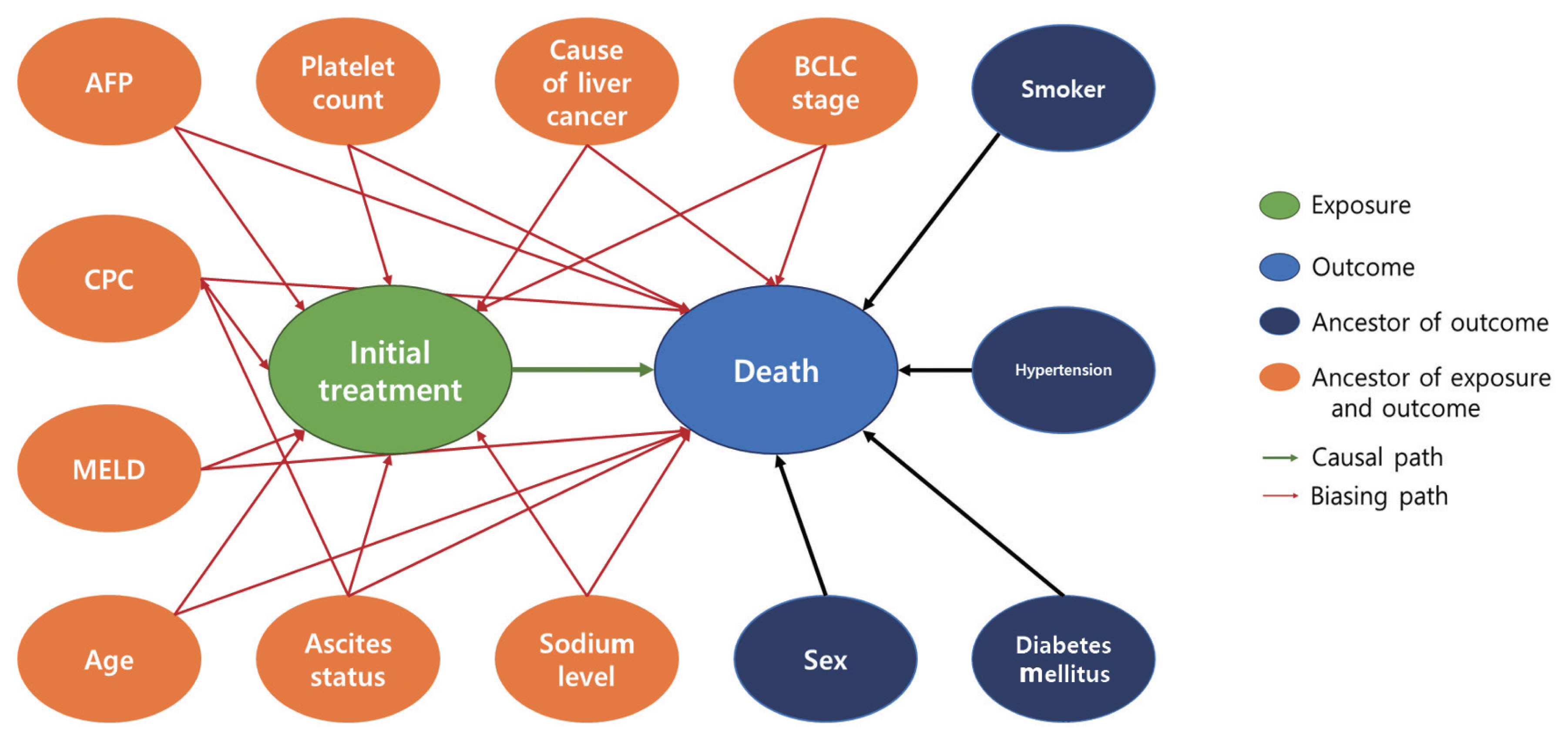
- Our study design was based on that of a previous study by Kim et al. [12] that compared the effect of radiofrequency ablation to surgical resection for hepatocellular carcinoma on survival. In this example, the effect of surgical resection and local ablation therapy on 3-year survival was compared based on standardization. Figure 1 shows the DAG for the causal relationships of all relevant variables for helping to determine the set of confounders used in standardization. DAGitty, which is the program used to create the DAGs in this study, offers several sets of confounders that can be adjusted for estimating the causal effect by exploiting Pearl’s backdoor criterion [13,14]. Therefore, the variables included in our study were age, ascites status (yes or no), Model for End-Stage Liver Disease (MELD) score, platelet count (0–50, 50–100, 100–150, >150 103/μL), sodium level (0–135, 135–145, >145 mmol/L), alpha-fetoprotein (AFP) level (0–200, 200–400, >400 ng/mL), Child-Pugh classification (A, B, C, U), and Barcelona Clinic Liver Cancer (BCLC) stage (0, A, B, C, D). We set a dichotomous variable (1=death, 0=survived) as the outcome. In addition, the causal estimands of treatment according to individuals’ BCLC stage were explored. Therefore, we considered using fitted models that included the interaction term between treatment and the BCLC stage variable. The final model was selected and consisted of variables with p-values of less than 0.05.
- This tutorial depicts 2 methods for estimating the causal effect of the treatment based on standardization using R software 4.0.5. One method used basic R functions only, while the other used the stdReg package in R. Hernán and Robins [4] introduced methods for estimating the ATE using basic R functions in cases when the outcome variable is a continuous measurement. Here, we show how causal estimands such as risk difference, risk ratio, and odds ratios were estimated for our dichotomous outcome. The stdReg package provides user-friendly functions for estimating the causal estimand based on standardization. We show how to compute the estimands using the stdGlm function and compare the package result with that of the first method.
- In the first method, a function for implementing the standardization for the causal estimands was created, and then bootstrapping was performed to calculate each estimand’s 95% confidence interval. The standardization function consisted of 4 parts. First, 2 datasets were duplicated by adding an index variable, and the copies of the datasets were combined. The first dataset was a copy of the original dataset (liver_syn_data0), and the second dataset (liver_syn_data2) included data on individuals that were identical to the original but with the treatment and death outcomes set to 0 and null, respectively. The third dataset (liver_syn_data3) included data on individuals that were identical to the original, but the treatment and death outcomes were set to 1 and null, respectively. The outcome variables in the 2 duplicated datasets were set as “NA” so that they would be ignored in the fitting step. Second, we fitted a logistic regression model in which the binary outcome was death within 3 years after the initial treatment prescription. Third, the probability of the event was calculated based on the fitted model. Therefore, the standardized probabilities of death were estimated for when all liver cancer patients underwent surgical resection and when all liver cancer patients underwent local ablation therapy. Finally, causal estimands such as risk difference, relative ratio, and odds ratio were computed.
- Next, the standardization function was applied to the boot function to perform bootstrapping with 1000 replications. The results of bootstrapping were used to construct 2 versions of the 95% confidence interval. The first version was referred to as the “normal-based confidence interval,” which used the standard error computed from the bootstrapped estimates. The second version used the 2.5% and 97.5% percentiles of the bootstrapped estimates as the left and right limits of the 95% confidence interval, respectively. In this tutorial, we report the first confidence interval in Tables 4 and 5 for brevity.
- The same causal estimands can also be computed using the stdReg package. The steps for applying the function in the stdReg package for estimating the estimands were simpler than the previous method. First, we fitted the same logistic regression model and applied the fitted model to the stdGlm function. The function required specifying the name of the exposure variable and the levels of exposure. Since the exposure of interest was the “treatment” variable, we set X=”treatment” and x=(0, 1, 1) in the stdGlm function. Each value within the parenthesis of the x argument indicated the minimum value, maximum value, and the unit of increment in order. Next, the estimates for the causal estimands using the summary function were presented. The summary function enabled estimation of the causal estimand with the standard error and 95% confidence interval by setting the contrast and reference options.
- The causal estimates from the standardization function and stdGlm function are compared in Table 4. The estimates and their 95% confidence intervals from the 2 methods were the same.
- Sensitivity analyses are generally performed to assess the robustness of findings in a study [15]. Although the set of confounders is selected from the DAG, various outcome models based on the same sets of confounders are possible by considering, for example, their interaction terms, and the causal estimates from different models are expected to reflect consistent results as long as they are close to the true model. For example, the fitted model for the standardization in our tutorial included the interaction term between the treatment and BCLC stage. If the fitted model properly controls the confounding effects, including additional interaction terms between the treatment and the other variables, the causal estimates should not change drastically.
- Table 5 shows the results of the sensitivity analysis. Different interaction terms were included in each model, and estimates from Tables 4 and 5 were compared to one another. The results of the sensitivity analysis support the robustness of our findings since the compared estimates were very similar.
- The R script for performing standardization on a subset of the population is shown in Supplemental Material 1. The method for estimating the subgroup causal effects was straightforward. In the standardization function, the procedure until the steps for fitting a logistic regression model was the same as estimating the whole population’s estimands. As such, individuals were selected from the subset of the population when averaging the probability of the event. When using the stdReg package, the estimands for the subset of the population can be computed by setting the subsetnew argument in the stdGlm function. The rest of the steps in both methods for estimating the subgroup causal effects were the same as those for the whole population. In the example, the subgroup consisted of individuals with a BCLC stage of A, and the results are presented in Supplemental Material 2. Sensitivity analyses were also performed for the subgroups, and the results are presented in Supplemental Material 3.
LIVER CANCER TREATMENT EXAMPLES
# Load libraries
   library (readxl)
   library (dplyr)
   library (boot)
   library (stdReg)
# Import liver synthetic data
    liver_syn_data1 <- read.csv (‘~/liver_syn_data.csv’)
# [1] Build function for standardization
   standardization <- function( data, indices ) {
   liver_syn_data0 <- data[indices, ]
   # [1]-1. data expansion
       # original
          liver_syn_data0$data.class <- ‘ori’
       # 2nd copy
          liver_syn_data2 <- liver_syn_data0 %>%
          mutate (data.class=‘T0’, Treatment=0, death=NA)
       # 3rd copy
          liver_syn_data3 <- liver_syn_data0 %>%
          mutate (data.class=‘T1’, Treatment=1, death=NA)
       # Combine all data
          onesample <- rbind ( liver_syn_data0, liver_syn_
             data2, liver_syn_data3)
   # [1]-2. Fit the model
      fit1 <-glm (death ~ Treatment * i_bclc+age+Liver_
         Cancer_Cause+MELD+cpc_cat+platelet_cat+
         Sodium_level+AFP_level+Ascites_status, family=
         ‘binomial’,data = onesample)
# Confounders in the dataset (i_bclc: BCLC stage; age: Age;
   Liver_Cancer_Cause: cause of liver cancer; MELD: MELD
   score; cpc_cat: child pugh classification; platelet_cat:
   Platelet count; Sodium_level: sodium level, AFP_level:
   alpha-fetoprotein; Ascites_status: ascites status)
   # [1]-3. Predict the outcome Y
      onesample$predicted.meanY 1 <- predict.glm (fit1,
         onesample, type=“response”)
      Y1T1=mean( onesample$predicted.meanY1
          [onesample$data.class==‘T1’])
      Y1T0=mean( onesample$predicted.meanY1
          [onesample$data.class==‘T0’])
   # [1]-4. Calculate the causal estimands
      ATE=Y1T1 - Y1T0 #Risk difference
      RR=Y1T1/Y1T0 #Relative ratio
      OR=(Y1T1/(1-Y1T1))/(Y1T0/(1-Y1T0)) #Odds ratio
      return(c(ATE, RR, OR))}
# [2] Generate confidence intervals
    # [2]-1. Calculate the 95% confidence interval
       set.seed(1234)
       results <- boot(data=liver_syn_data1, statistic=
          standardization, R=1,000, parallel=“multicore”)
       se <- c(sd(results$t[, 1]), sd(results$t[, 2]),
        sd(results$t[, 3]))
     mean <- results$t0
# 95% normal confidence interval using se
      ll1 <- mean - qnorm(0.975) * se
      ul1 <- mean + qnorm(0.975) * se
# 95% percentile confidence interval
      ll2 <- c (quantile (results$t[,1], 0.025), quantile
         (results$t[,2], 0.025), quantile (results$t[,3], 0.025))
      ul2 <- c (quantile (results$t[,1], 0.975), quantile
         (results$t[,2], 0.975), quantile (results$t[,3], 0.975))
  # [2]-2. Present the result
      bootstrap <-data.frame(cbind(c(“ATE”, “RR”, “OR”), round
          (mean, 4), round (se, 4), round (ll1, 4), round (ul1, 4),
          round (ll2, 4), round (ul2, 4)), row.names=NULL)
      colnames (bootstrap) <- c(“Estimand”, “mean”, “se”,
          “Lower1”, “Upper1”, “Lower2”, “Upper2”)
# [3] Standardization using the stdReg package
   fit1 <-glm (death ~ Treatment * i_bclc+age+Liver_
      Cancer_Cause+MELD+cpc_cat+platelet_cat+
      Sodium_level+AFP_level+Ascites_status, family=
      ‘binomial’, data=liver_syn_data1)
   fit.std <- stdGlm (fit=fit1, data=liver_syn_data1,
      X=“Treatment”, x= seq (0,1,1))
   summary (fit.std, contrast=‘difference’, reference=0)
      #Risk difference
   summary (fit.std, contrast=‘ratio’, reference=0)
      #Relative ratio
   summary (fit.std, transform=‘odds’, contrast=“ratio”,
      reference=0) #Odds ratio
- Standardization is traditionally used in epidemiology when reporting the specific rate or ratio of a disease, such as the age-standardized incidence rate and the standardized mortality ratio [16]. The application of standardization would remove the confounding effect [17]. For example, a country with a population distribution that is skewed toward the elderly would always show a high cancer incidence. In these cases, using the age-standardized incidence rate of cancer would remove the confounding effect of the age variable.
- Standardization in causal inference answers the causal question based on the potential outcome if everyone is either treated or untreated. Causal inference based on observational studies is difficult since the causal estimand is not fully identifiable without having to make a strong assumption. The observational study must also have conditions that are similar to those of a conditional randomized experiment. However, the required conditional exchangeability between treated and untreated subjects cannot be proven by data and can only be examined using subject matter knowledge.
- Our tutorial demonstrated how standardization is implemented for estimating various causal estimands. Before fitting a regression model, creating a DAG is important since it guides the systematic selection of the potential confounders that will be included in a model. In particular, nodes and arrows in a DAG are drawn based on background knowledge [18], and different versions of a DAG can be used for sensitivity analysis. Consistent results from different versions of DAGs indicate a higher degree of confidence in the causal effect estimation. Additional sensitivity analysis under unmeasured confounding may also be performed using subject matter knowledge.
- Standardization is simply a method for estimating the causal estimand of interest. Other methods such as inverse probability weighting, propensity score matching, and instrumental variable methods are some alternatives with different assumptions. Inverse probability weighting is usually compared to standardization when estimating the causal estimand [19]. The key difference between the two methods is based on which parts are modeled. Inverse probability weighting models the treatment using Pr[T=t|C=c], while standardization models the outcome using Pr[Y=1|T=t, C=c]. The propensity score matching method estimates the causal estimands from exposed and unexposed groups that are matched based on the propensity score [20]. Instrumental variables, associated with treatment but not associated with outcomes, as well as confounders, can be used to estimate the estimands even when confounding variables are not measured. However, all methods require either the conditional exchangeability condition or its corresponding untestable conditions. Therefore, researchers should be fully aware that causal inference from an observational study cannot replace causal inference from an RCT. Conditional exchangeability is an untestable assumption in an observational study, whereas in an RCT, conditional exchangeability holds true in practice.
- Ethics Statement
- No ethics approval and consent to participate was necessary since we used a synthetic data.
DISCUSSION AND CONCLUSION
SUPPLEMENTAL MATERIALS
Supplemental Material 1.
Supplemental Material 2.
Supplemental Material 3.
ACKNOWLEDGEMENTS
-
CONFLICT OF INTEREST
The authors have no conflicts of interest associated with the material presented in this paper.
-
AUTHOR CONTRIBUTIONS
Both authors contributed equally to conceiving the study, analyzing the data, and writing this paper.
-
FUNDING
This study was supported by the National Research Foundation of Korea (NRF) grant funded by the Korea government (MSIT) (No.2021R1A2C1014409).
Notes
| Estimand | Model 11 | Model 22 | Model 33 |
|---|---|---|---|
| Risk difference | 0.02 (−0.01, 0.04) | 0.02 (−0.01, 0.04) | 0.02 (−0.01, 0.04) |
| Relative risk | 1.09 (0.94, 1.25) | 1.10 (0.94, 1.25) | 1.10 (0.94, 1.25) |
| Odds ratio | 1.12 (0.92, 1.32) | 1.12 (0.92, 1.32) | 1.12 (0.92, 1.32) |
Values are presented as estimate (95% confidence interval).
BCLC, Barcelona Clinic Liver Cancer.
1 Interaction term between treatment, BCLC stage, and alpha-fetoprotein level and other confounders are included in the model.
2 Interaction term between treatment, BCLC stage, and cause of liver cancer and other confounders are included in the model.
3 Interaction term between treatment and Child-Pugh classification and other confounders are included in the model.
- 1. Concato J, Shah N, Horwitz RI. Randomized, controlled trials, observational studies, and the hierarchy of research designs. N Engl J Med 2000;342(25):1887-1892ArticlePubMedPMC
- 2. Altman N, Krzywinski M. Association, correlation and causation. Nat Methods 2015;12(10):899-900ArticlePubMed
- 3. Hernán MA, Hernández-Díaz S, Werler MM, Mitchell AA. Causal knowledge as a prerequisite for confounding evaluation: an application to birth defects epidemiology. Am J Epidemiol 2002;155(2):176-184ArticlePubMed
- 4. Hernán MA, Robins JM. Causal inference: what If; [cited 2021 Oct 1]. Available from: https://cdn1.sph.harvard.edu/wp-content/uploads/sites/1268/2021/03/ciwhatif_hernanrobins_30mar21.pdf
- 5. Sjölander A. Regression standardization with the R package stdReg. Eur J Epidemiol 2016;31(6):563-574ArticlePubMed
- 6. Hernán MA, Hernández-Díaz S, Robins JM. A structural approach to selection bias. Epidemiology 2004;15(5):615-625ArticlePubMed
- 7. Cole SR, Platt RW, Schisterman EF, Chu H, Westreich D, Richardson D, et al. Illustrating bias due to conditioning on a collider. Int J Epidemiol 2010;39(2):417-420ArticlePubMed
- 8. Shrier I, Platt RW. Reducing bias through directed acyclic graphs. BMC Med Res Methodol 2008;8: 70ArticlePubMedPMC
- 9. Westreich D, Cole SR. Invited commentary: positivity in practice. Am J Epidemiol 2010;171(6):674-677ArticlePubMedPMC
- 10. Song BG, Kim MJ, Sinn DH, Kang W, Gwak GY, Paik YH, et al. A comparison of factors associated with the temporal improvement in the overall survival of BCLC stage 0 hepatocellular carcinoma patients. Dig Liver Dis 2021;53(2):210-215ArticlePubMed
- 11. Nowok B, Raab GM, Dibben C. synthpop: Bespoke creation of synthetic data in R. J Stat Softw 2016;74(11):1-26
- 12. Kim GA, Shim JH, Kim MJ, Kim SY, Won HJ, Shin YM, et al. Radiofrequency ablation as an alternative to hepatic resection for single small hepatocellular carcinomas. Br J Surg 2016;103(1):126-135ArticlePubMed
- 13. Textor J. Drawing and analyzing causal DAGs with DAGitty; arXiv [Preprint]. 2015 [cited 2021 Oct 22]. Available from: https://arxiv.org/pdf/1508.04633.pdf
- 14. Pearl Judea, Glymour Madelyn, Jewell Nicholas P. Causal inference in statistics: a primer. Chichester: Wiley; 2016. p. 1-136
- 15. Thabane L, Mbuagbaw L, Zhang S, Samaan Z, Marcucci M, Ye C, et al. A tutorial on sensitivity analyses in clinical trials: the what, why, when and how. BMC Med Res Methodol 2013;13: 92ArticlePubMedPMC
- 16. Gharibzadeh S, Mohammad K, Rahimiforoushani A, Amouzegar A, Mansournia MA. Standardization as a tool for causal inference in medical research. Arch Iran Med 2016;19(9):666-670PubMed
- 17. Keiding N, Clayton D. Standardization and control for confounding in observational studies: a historical perspective. Stat Sci 2014;29(4):529-558Article
- 18. Ferguson KD, McCann M, Katikireddi SV, Thomson H, Green MJ, Smith DJ, et al. Evidence synthesis for constructing directed acyclic graphs (ESC-DAGs): a novel and systematic method for building directed acyclic graphs. Int J Epidemiol 2020;49(1):322-329ArticlePubMed
- 19. Hernán MA, Robins JM. Estimating causal effects from epidemiological data. J Epidemiol Community Health 2006;60(7):578-586ArticlePubMedPMC
- 20. Stuart EA. Matching methods for causal inference: a review and a look forward. Stat Sci 2010;25(1):1-21ArticlePubMedPMC
REFERENCES
Figure & Data
References
Citations
- Improved Clinical Outcomes With Early Anti-Tumour Necrosis Factor Alpha Therapy in Children With Newly Diagnosed Crohn’s Disease: Real-world Data from the International Prospective PIBD-SETQuality Inception Cohort Study
Renz C W Klomberg, Hella C van der Wal, Martine A Aardoom, Polychronis Kemos, Dimitris Rizopoulos, Frank M Ruemmele, Mohammed Charrout, Hankje C Escher, Nicholas M Croft, Lissy de Ridder, Ivan D Milovanovich, James J Ashton, Paul Henderson, Oren Ledder, T
Journal of Crohn's and Colitis.2024; 18(5): 738. CrossRef - Homologous and Heterologous Prime-Boost Vaccination: Impact on Clinical Severity of SARS-CoV-2 Omicron Infection among Hospitalized COVID-19 Patients in Belgium
Marjan Meurisse, Lucy Catteau, Joris A. F. van Loenhout, Toon Braeye, Laurane De Mot, Ben Serrien, Koen Blot, Emilie Cauët, Herman Van Oyen, Lize Cuypers, Annie Robert, Nina Van Goethem
Vaccines.2023; 11(2): 378. CrossRef
 PubReader
 ePub Link
 Cite
Cite

